Extending the Model in R
Adding a disease stage
Continuing in R from the last session, we will now extend the disease
to include an additional, less-infectious, semi-recovering stage, which
will come after I, and be called IR. We do this by inserting a new
stage, named “IR”, at index 2, with beta value 0.2, and progress
value 0.1
> lurgy$insert(2, name="IR", beta=0.2, progress=0.1)
> print(lurgy)

* Disease: lurgy
* stage: ['E', 'I', 'IR', 'R']
* mapping: ['E', 'I', 'IR', 'R']
* beta: [0.0, 0.8, 0.2, 0.0]
* progress: [0.25, 0.25, 0.1, 0.0]
* too_ill_to_move: [0.0, 0.0, 0.0, 0.0]
* start_symptom: 2
Note
MetaWards is a Python program, so the index is counted from 0. Index 0 is E, index 1 is I and (before this call), index 2 was R. Inserting at index 2 will insert IR between I and R
We can now run the model using metawards.run(). This time we will
set silent to TRUE so that it doesn’t print so much output
to the screen.
> results <- metawards$run(model=home, disease=lurgy,
                           additional=100, silent=TRUE)

 ━━━━━━━━━━━━━━━━━━━━━━━━━━━━━━━━━━━━━ INFO ━━━━━━━━━━━━━━━━━━━━━━━━━━━━━━━━━━━━━
 Writing output to directory ./output_n81uzd7l

 ━━━━━━━━━━━━━━━━━━━━━━━━━━━━━━━━━━━━━━━━━━━━━━━━━━━━━━━━━━━━━━━━━━━━━━━━━━━━━━━━
Note
All of the output is written to the (randomly) named output directory
indicated, e.g. for me to output_n81uzd7l. The full log of the run
is recorded in the file called console.log.bz2 which is in
this directory.
We can now process and plot the results identically to before, e.g.
> results <- read.csv(results)
> results <- results %>%
     pivot_longer(c("S", "E", "I", "R"),
     names_to = "stage", values_to = "count")
> ggplot(data = results,
         mapping = aes(x=day, y=count, color=stage)) + geom_line()
Repeating a run
MetaWards model runs are stochastic, meaning that they use random numbers. While each individual run is reproducible (given the same random number seed and number of processor threads), it is best to run multiple runs so that you can look at averages.
You can perform multiple runs using the repeats argument, e.g.
to perform four runs, you should type;
> results <- metawards$run(model=home, disease=lurgy,
                           additional=100, silent=TRUE, repeats=4)
If you look at the results, you will that there is a repeat column, which indexes each run with a repeat number, e.g.
> results <- read.csv(results)
> print(results)

    fingerprint repeat. day       date     S    E    I   IR    R IW SCALE_UV
 1       REPEAT       1   0 2020-07-21 10000    0    0    0    0  0        1
 2       REPEAT       1   1 2020-07-22  9900   82   18    0    0  1        1
 3       REPEAT       1   2 2020-07-23  9887   81   27    5    0  1        1
 4       REPEAT       1   3 2020-07-24  9869   77   44    9    1  1        1
 5       REPEAT       1   4 2020-07-25  9826  102   50   20    2  1        1
 6       REPEAT       1   5 2020-07-26  9783  113   67   34    3  1        1
 7       REPEAT       1   6 2020-07-27  9724  149   73   48    6  1        1
 8       REPEAT       1   7 2020-07-28  9653  174   96   64   13  1        1
 9       REPEAT       1   8 2020-07-29  9573  209  118   80   20  1        1
 10      REPEAT       1   9 2020-07-30  9472  254  145   99   30  1        1
Note
Because repeat is a keyword in R, the column is automatically renamed
as repeat.
We can pivot and graph these runs using;
> results <- results %>%
     pivot_longer(c("S", "E", "I", "IR", "R"),
     names_to = "stage", values_to = "count")
> ggplot(data = results,
         mapping = aes(x=day, y=count, color=stage)) + geom_point()
Note
We have used geom_point() rather than geom_line() as this better
shows the different runs. With a bit more R you could adjust the
point shape to match the repeat number.
You should get a result that looks something like this;
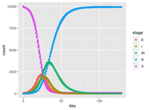
From this you can see the build-up of individuals in the green long recovery (IR) stage.
Adding more wards
Next, we will extend the model by adding more wards. We will model home, work and school, so let’s now add the work and school wards.
> work <- metawards$Ward("work")
> school <- metawards$Ward("school")
We will now add some workers who will make daily, predictable movements from home to work or school.
> home$add_workers(7500, destination=work)
> home$add_workers(5000, destination=school)
Note
The term worker is very broad in MetaWards. It means any individual that make regular, predictable movements each day. In this case, it refers to workers, teachers and students.
Next we need to combine these individual Ward objects
into a single Wards that represents the entire network.
> network <- metawards$Wards()
> network$add(home)
> network$add(work)
> network$add(school)
Running the model
We can now run the model. In this case, we want to seed the infection in
the home ward, so we need to pass this name into the additional
parameter.
> results <- metawards$run(disease=lurgy, model=network,
                           additional="1, 100, home")
Note
The format is day number (in this case seed on day 1), then number to seed (seeding 100 infections), then ward name or number (in this case, home)
You will see a lot of output. MetaWards does print a table to confirm the seeding, e.g.
┏━━━━━┳━━━━━━━━━━━━━┳━━━━━━━━━━━━━━━━━━━━━━━━━━━━━━━━━━━━━━━━━━━━━━┳━━━━━━━━━━━┓
┃ Day ┃ Demographic ┃                     Ward                     ┃  Number   ┃
┃     ┃             ┃                                              ┃  seeded   ┃
┡━━━━━╇━━━━━━━━━━━━━╇━━━━━━━━━━━━━━━━━━━━━━━━━━━━━━━━━━━━━━━━━━━━━━╇━━━━━━━━━━━┩
│  1  │    None     │ 1 : WardInfo(name='home', alternate_names=,  │    100    │
│     │             │   code='', alternate_codes=, authority='',   │           │
│     │             │        authority_code='', region='',         │           │
│     │             │               region_code='')                │           │
└─────┴─────────────┴──────────────────────────────────────────────┴───────────┘
The results can be processed and visualised as before, e.g.
> results <- read.csv(results)
> results <- results %>%
     pivot_longer(c("S", "E", "I", "IR", "R"),
     names_to = "stage", values_to = "count")
> ggplot(data = results,
         mapping = aes(x=day, y=count, color=stage)) + geom_point()
Complete code
The complete R code for this part of the getting started guide is re-copied below (this continues from the code in the last part);
# add the IR stage between the I and R stages
lurgy$insert(2, name="IR", beta=0.2, progress=0.1)

# create the network of home, work and school wards
work <- metawards$Ward("work")
school <- metawards$Ward("school")
network <- metawards$Wards()

home$add_workers(7500, destination=work)
home$add_workers(5000, destination=school)

network$add(home)
network$add(work)
network$add(school)

# run the model using the updated disease and network
results <- metawards$run(disease=lurgy, model=network,
                         additional="1, 100, home")

# plot the resulting trajectory
results <- read.csv(results)
results <- results %>%
     pivot_longer(c("S", "E", "I", "IR", "R"),
     names_to = "stage", values_to = "count")
ggplot(data = results,
       mapping = aes(x=day, y=count, color=stage)) + geom_point()