Getting Started in the Console

Prerequisites

First, you need to open the terminal (or console or command prompt) and type;

metawards --version

You should see that MetaWards version information is printed to the screen. If not, then you need to install MetaWards.

Note

The output should show that MetaWardsData has been found. If you have not installed MetaWardsData then you need to install it by following these instructions.

You also need to be able to use a text editor, e.g. notepad, vim, emacs, nano or pico. This quick start will use nano. Please use the editor that you prefer.

Creating the disease

You should now be at an open terminal.

To run a simulation you need to define the Disease that you want to model. MetaWards implements a SEIR-style model, but you have complete control to define as many (or few) stages as you wish.

First, we will create a disease, which we will call lurgy, that will consist of four stages: S, E, I and R. While you can use the Python or R API to create this model in Python or R, you can also write the required JSON data file directly at the console. Create a new text file called lurgy.json, e.g. by typing;

nano lurgy.json

and type in the below;

{
  "name": "lurgy",
  "stage": ["E", "I", "R"],
  "beta": [0.0, 0.8, 0.0],
  "progress": [0.5, 0.25, 0.0]
}

This defines the three stages, “E”, “I” and “R”. You don’t define the “S” stage, as the model starts with a set of susceptible individuals by default.

The beta (infectivity) parameters are set such that individuals are not infectious during the latent (“E”) stage or recovered (“R”) stage (beta equals 0), but are quite infectious in the “I” stage (beta equals 0.8).

The progress parameter is set so that individuals progress quickly through the “E” stage (progress equals 0.5, meaning that 50% of individuals move to the next stage each day), while progress through the “I” stage is slower (progress equals 0.25). The progress value for the “R” stage must be 0, as once recovered, the individual no longer moves through the model.

Creating the wards (network)

Next, you need to define the wards (network) that will contain the individuals who will experience the model outbreak.

We will first start with a single ward, called home, in a file called network.json.

[
  {
    "info": {
        "name": "home"
    },
    "num_players": 10000
  }
]

MetaWards works by assigning individuals as either workers or players. The difference is that workers make fixed (predictable) movements between different wards each day, while players make random movements. Since we have just a single ward, called “home”, and we start by populating it with 10,000 players.

Running the model

Now we have a disease and a network, we can now model an outbreak. To do this, we will run the metawards program directly.

metawards --disease lurgy.json --model network.json

This will print a lot to the screen. The key lines are these;

━━━━━━━━━━━━━━━━━━━━━━━━━━━━━━━━━━━━ Day 0 ━━━━━━━━━━━━━━━━━━━━━━━━━━━━━━━━━━━━━
S: 10000  E: 0  I: 0  R: 0  IW: 0  POPULATION: 10000

━━━━━━━━━━━━━━━━━━━━━━━━━━━━━━━━━━━━ Day 1 ━━━━━━━━━━━━━━━━━━━━━━━━━━━━━━━━━━━━━
S: 10000  E: 0  I: 0  R: 0  IW: 0  POPULATION: 10000
Number of infections: 0

━━━━━━━━━━━━━━━━━━━━━━━━━━━━━━━━━━━━ Day 2 ━━━━━━━━━━━━━━━━━━━━━━━━━━━━━━━━━━━━━
S: 10000  E: 0  I: 0  R: 0  IW: 0  POPULATION: 10000
Number of infections: 0

━━━━━━━━━━━━━━━━━━━━━━━━━━━━━━━━━━━━ Day 3 ━━━━━━━━━━━━━━━━━━━━━━━━━━━━━━━━━━━━━
S: 10000  E: 0  I: 0  R: 0  IW: 0  POPULATION: 10000
Number of infections: 0

━━━━━━━━━━━━━━━━━━━━━━━━━━━━━━━━━━━━ Day 4 ━━━━━━━━━━━━━━━━━━━━━━━━━━━━━━━━━━━━━
S: 10000  E: 0  I: 0  R: 0  IW: 0  POPULATION: 10000
Number of infections: 0

━━━━━━━━━━━━━━━━━━━━━━━━━━━━━━━━━━━━ Day 5 ━━━━━━━━━━━━━━━━━━━━━━━━━━━━━━━━━━━━━
S: 10000  E: 0  I: 0  R: 0  IW: 0  POPULATION: 10000
Number of infections: 0
Ending on day 5

This shows the number of people in the different stages of the outbreak. In this case, there was no infection seeded, and so the number of infections remained zero.

Seeding the outbreak

We need to seed the outbreak with some additional seeds. We do this using the additional option. This can be very powerful (e.g. adding seeds at different days, different wards etc.), but at its simplest, it is just the number of initial infections on the first day in the first ward. We will start with 100 initial infections;

metawards --disease lurgy.json --model network.json --additonal 100

Note

MetaWards writes its output to a directory called output. You can change this using the --output argument. By default, MetaWards will check before overwriting output. To remove this check, pass in the --force-overwrite-output option.

Now you get a lot more output, e.g. for me the outbreak runs for 71 days.

━━━━━━━━━━━━━━━━━━━━━━━━━━━━━━━━━━━━━━━━━━━━━━━━━━━ Day 67 ━━━━━━━━━━━━━━━━━━━━━━━━━━━━━━━━━━━━━━━━━━━━━━━━━━━
S: 520  E: 1  I: 1  R: 9478  IW: 1  POPULATION: 10000
Number of infections: 2

━━━━━━━━━━━━━━━━━━━━━━━━━━━━━━━━━━━━━━━━━━━━━━━━━━━ Day 68 ━━━━━━━━━━━━━━━━━━━━━━━━━━━━━━━━━━━━━━━━━━━━━━━━━━━
S: 520  E: 0  I: 1  R: 9479  IW: 0  POPULATION: 10000
Number of infections: 1

━━━━━━━━━━━━━━━━━━━━━━━━━━━━━━━━━━━━━━━━━━━━━━━━━━━ Day 69 ━━━━━━━━━━━━━━━━━━━━━━━━━━━━━━━━━━━━━━━━━━━━━━━━━━━
S: 520  E: 0  I: 1  R: 9479  IW: 0  POPULATION: 10000
Number of infections: 1

━━━━━━━━━━━━━━━━━━━━━━━━━━━━━━━━━━━━━━━━━━━━━━━━━━━ Day 70 ━━━━━━━━━━━━━━━━━━━━━━━━━━━━━━━━━━━━━━━━━━━━━━━━━━━
S: 520  E: 0  I: 1  R: 9479  IW: 0  POPULATION: 10000
Number of infections: 1

━━━━━━━━━━━━━━━━━━━━━━━━━━━━━━━━━━━━━━━━━━━━━━━━━━━ Day 71 ━━━━━━━━━━━━━━━━━━━━━━━━━━━━━━━━━━━━━━━━━━━━━━━━━━━
S: 520  E: 0  I: 0  R: 9480  IW: 0  POPULATION: 10000
Number of infections: 0
Ending on day 71

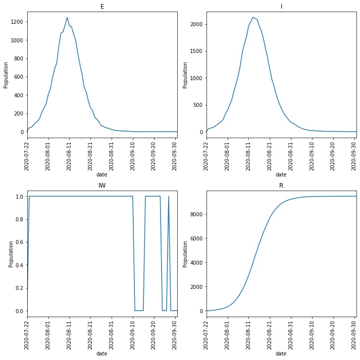
Visualising the results

The output is written to the output directory. In here is a comma-separated file called results.csv.bz2 (MetaWards automatically bzip2 compresses most files to save space). This contains the full trajectory, e.g. reading this via bunzip2 -kc output/results.csv.bz2 should show something that starts with;

fingerprint,repeat,day,date,S,E,I,R,IW,SCALE_UV
REPEAT,1,0,2020-07-22,10000,0,0,0,0,1.0
REPEAT,1,1,2020-07-23,9900,45,55,0,1,1.0
REPEAT,1,2,2020-07-24,9867,48,66,19,1,1.0
REPEAT,1,3,2020-07-25,9818,71,76,35,1,1.0
REPEAT,1,4,2020-07-26,9755,98,99,48,1,1.0
REPEAT,1,5,2020-07-27,9685,112,129,74,1,1.0
REPEAT,1,6,2020-07-28,9587,151,158,104,1,1.0
REPEAT,1,7,2020-07-29,9461,213,185,141,1,1.0
REPEAT,1,8,2020-07-30,9317,260,235,188,1,1.0
REPEAT,1,9,2020-07-31,9130,300,326,244,1,1.0
REPEAT,1,10,2020-08-01,8869,406,399,326,1,1.0

We can visualise the data by loading into Python (pandas), R or Excel. MetaWards also comes with a quick plotting program called metawards-plot. Use this to visualise the results using;

metawards-plot -i output/results.csv.bz2

Note

This program may prompt you to install additional Python modules, e.g. pandas and matplotlib

This should produce a resulting image (output/overview.png) that looks something like this;