Disease pathways and stages
Up to this point, every individual modelled in metawards progresses
through the same stages of the same disease pathway. This pathway
is defined in the disease file (e.g. lurgy4.json) and progresses
an individual from being susceptible to infection (S) to the
final stage of the disease (normally called R to represent individuals
who are removed from the outbreak).
Stages of the lurgy
For the lurgy, the disease stages are;
S- this is the starting point of all individualsStage 0- this is a holding state. Individuals are moved into this state as soon as they are infected. This is used to record internally inmetawardsto record new infections each day. Theprogressvalue for this state (progress[0]) should be1.0, to show that individuals will immediately progress toStage 1(the latent,Estate) the next day. Equally, thebetavalue for this state (beta[0]) should be0.0as individuals in this state should not contribute to the force of infection.Stage 1- this is the latent orEstate. Individuals are held in this state with a duration defined byprogress[1]. Thebeta[1]value should be0.0as latent individuals are not infectious and should not thus contribute to the force of infection.Stages 2-4- these are the infected orIstates. The lurgy has three such states, withStage 2(orI1) representing the asymptomatic infectious state (lowbetabut zerotoo_ill_to_move), thenStage 3(orI2) representing the initial symptomatic state (mediumbetaand mediumtoo_ill_to_move), andStage 4(orI3) representing the highly symptomatic state (mediumbetaand hightoo_ill_to_move).Stage 5- this is the removed orRstate. Individuals in this state cannot infect others, and sobetais0.0andtoo_ill_to_moveis1.0(no need to model movements of non-infectious or infectable individuals). Theprogressvalue is0.0as, once removed, individuals remain in this stage for the remainder of the model run.
Modelling a fraction of asymptomatic super-spreaders
It is really useful to have the ability to model different demographics following different disease pathways. For example, up to now we have modelled the lurgy as having an asymptomatic infectious phase which everyone will move through. However, in reality, only a small proportion of those infected by the lurgy will become these asymptomatic “super-spreaders”. We would like to investigate how the percentage of these super-spreaders, and their mobility and infectivity affects the progression of the outbreak. To do this, we will create two demographics;
home, which will contain a population who do not progress through the asymptomatic infectious stage, and
super, which will contain a population of super-spreaders who do move through the asymptomatic infectious phase.
To start, we need to create disease files for the home and super
demographics. Do this by creating two files, first lurgy_home.json that
should contain;
{ "name"             : "The Lurgy",
  "version"          : "June 2nd 2020",
  "author(s)"        : "Christopher Woods",
  "contact(s)"       : "christopher.woods@bristol.ac.uk",
  "reference(s)"     : "Completely ficticious disease - no references",
  "beta"             : [0.0, 0.0, 0.5, 0.5, 0.0],
  "progress"         : [1.0, 1.0, 0.5, 0.5, 0.0],
  "too_ill_to_move"  : [0.0, 0.0, 0.5, 0.8, 1.0],
  "contrib_foi"      : [1.0, 1.0, 1.0, 1.0, 0.0]
}
and lurgy_super.json that should contain;
{ "name"             : "The Lurgy",
  "version"          : "June 2nd 2020",
  "author(s)"        : "Christopher Woods",
  "contact(s)"       : "christopher.woods@bristol.ac.uk",
  "reference(s)"     : "Completely ficticious disease - no references",
  "beta"             : [0.0, 0.0, 0.8, 0.2, 0.1, 0.0],
  "progress"         : [1.0, 1.0, 0.5, 0.5, 0.5, 0.0],
  "too_ill_to_move"  : [0.0, 0.0, 0.0, 0.1, 0.0, 1.0],
  "contrib_foi"      : [1.0, 1.0, 1.0, 1.0, 1.0, 0.0]
}
In these files we have removed the asymptomatic infectious phase from the
home demographic, and then changed the super demographic to
experience a highly infectious asymptomatic stage, followed by a
very mild disease of decreasing infectiousness.
Next, we need to create the demographics.json file that should contain;
{
    "demographics" : ["home", "super"],
    "work_ratios"  : [ 0.9, 0.1 ],
    "play_ratios"  : [ 0.9, 0.1 ],
    "diseases"     : [ null, "lurgy_super" ]
}
This describes the two demographics, with 90% of individuals in the
home demographic, and 10% in the super demographic. The new
line here, disease_stages, specifies the file for the disease stages
for each demographic, e.g. home will follow the default disease, while
super will follow lurgy_super.
Note
null in a json file means “nothing”. In this case, “nothing” means
that the home demographic should use the disease parameters from
the global disease file set by the user.
Run metawards using the command;
metawards -d lurgy_home -D demographics.json --mixer mix_evenly -a ExtraSeedsLondon.dat
Note
Here we set the global disease file, via -d lurgy_home to lurgy_home.
This will be used by the home demographic. In theory we could have
specified lurgy_home directly in the demographics.json file,
but this would mean we would have to specify it twice, once there and once
globally. It is better to define things once only, as this leads to fewer
bugs.
Note
Note that we are using mix_evenly().
This may not be the right choice depending on how we want the
population dynamics to mix, e.g.
mix_evenly_single_population() or
mix_evenly_multi_population() may
be a better choice. See here for more information.
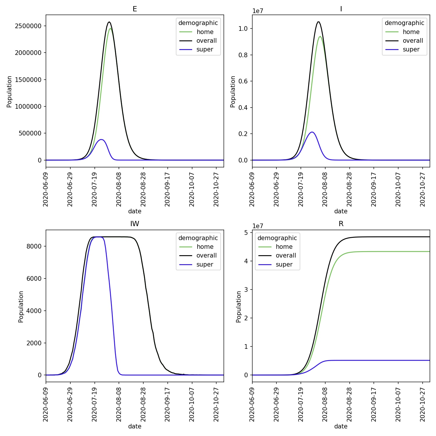
You should see that the disease spreads quickly via the super-spreaders, with all, or almost all becoming infected. You can see this in the demographics plot, produced via;
metawards-plot -i output/trajectory.csv.bz2
You should see something similar to this, which shows that the infection burns quickly through the super-spreader demographic, moving through that entire demographic in just a couple of months.
Note
It is counter-intuitive that the super-spreaders are all infected quickly,
and complete the outbreak long before the general population. This is
due to the model setup. The super-spreaders all interact with each other
within their demographic, and so, as their beta value is high,
there is a high probability that they will infect each other quickly.
Their limited population naturally means that it takes less time until
all members of the this population are infected.
While not wholly realistic, this does make some practical sense, as real super-spreaders will go about their normal day during an outbreak as they do not noticeably become ill. As they will continue normally, it could make sense that they outbreak could burn through that population quickly, until the point where there are few remaining. Meanwhile, the larger, more general population experiences a slower outbreak.
One way to counter this effect would be to use an interaction matrix to slow down the rate of infection in the super-spreader demographic. This would reflect the reality that super-spreaders are more dispersed, and so less likely to interact with one another than with members of the general population. An interaction matrix of, e.g. (1, 1, 1, 0.5) may thus be appropriate, although data fitting would be needed to find the exact values.